11 minutes
Machine Learning in Nmap
Notes
- The original post has been published on the Amossys blog
- I present some pieces of codes which are originally commented by their authors. I keep authors’ comments under the format
/* comments */while my own comments use the format// comments. - I use the version 7.70SVN of
nmap.
First discovery
After installing a basic Raspbian on my RPi, I also decided to add nmap to the system. Not so hard… but I was quite amazed.
$ sudo apt install nmap
...
The following additional packages will be installed:
  liblinear3 liblua5.3-0 ndiff python-bs4 python-html5lib python-lxml
  python-webencodings
...
The package manager demands other packages, especially lua and python stuff. Ok, why not, but why liblinear3 ?!
Actually, liblinear is a library for linear classification. Hum… it looks weird, so I decided to go deeper!
Deep learning
Sorry for the pun, but there is not any neural network behind that.
Looking at the code of liblinear, available on GitHub, we basically learn the following:
LIBLINEAR is a simple package for solving large-scale regularized linear
classification and regression. It currently supports
- L2-regularized logistic regression/L2-loss support vector classification/L1-loss support vector classification
- L1-regularized L2-loss support vector classification/L1-regularized logistic regression
- L2-regularized L2-loss support vector regression/L1-loss support vector regression.
In a word, it can do three things:
- logistic regression
- support vector classification
- support vector regression
Even if the first technique aimed to fit data to a model, it is mainly used to perform binary classification. The code boils down to few files:
linear.htron.h
liblinear won the ICML 2008 large-scale learning challenge and has been used to win the KDD Cup 2010 (see https://www.csie.ntu.edu.tw/~cjlin/liblinear/).Coming back to Nmap
Now, the goal is to look for liblinear inside the nmap code (about 85Mb).
$ git clone https://github.com/nmap/nmap.git
The natural idea is to grep “linear.h” in the folder.
$ cd nmap
$ grep -r linear.h
liblinear/Makefile:linear.o: linear.cpp linear.h
liblinear/liblinear.vcxproj:    <ClInclude Include="linear.h" />
liblinear/Makefile.win:linear.obj: linear.cpp linear.h
liblinear/Makefile.win:lib: linear.cpp linear.h linear.def tron.obj
liblinear/linear.cpp:#include "linear.h"
liblinear/predict.c:#include "linear.h"
liblinear/train.c:#include "linear.h"
FPModel.cc:#include "linear.h"
configure.ac:  AC_CHECK_HEADERS([linear.h],
FPEngine.cc:#include "linear.h"
configure:  for ac_header in linear.h
configure:  ac_fn_c_check_header_mongrel "$LINENO" "linear.h" "ac_cv_header_linear_h" "$ac_includes_default"
configure:if test "x$ac_cv_header_linear_h" = xyes; then :
The result shows a dozen of occurrences. The “configure” file is not interesting. The occurrences inside liblinear/ are not relevant as nmap stores the library code inside it. Finally we have two source code files FPModel.cc and FPEngine.cc which draw our attention (‘FP’ means ‘finger-printing’).
In the folder we can also find two headers FPModel.h and FPEngine.h.
In FPModel.h, five objects are introduced.
extern struct model FPModel;
extern double FPscale[][2];
extern double FPmean[][695];
extern double FPvariance[][695];
extern FingerMatch FPmatches[];
The FPEngine.h is quite richer and notably defines an FPEngine object
/* This class is the generic fingerprinting engine. */
class FPEngine {

protected:
  size_t osgroup_size;

public:
  FPEngine();
  ~FPEngine();
  void reset();
  virtual int os_scan(std::vector<Target *> &Targets) = 0;
  const char *bpf_filter(std::vector<Target *> &Targets);

};
Looking at the methods of FPEngine, we start to understand the purpose of liblinear: OS detection, which is a very nice and powerful feature in practice, isn’t it?
A fingerprint model
While the header FPModel.h is rather small, the objects it declares are really heavy! They are all implemented in FPModel.cc.
In particular the FPModel structure is an instance of a model defined in liblinear.h:
struct model
{
	struct parameter param;
	int nr_class;		/* number of classes */
	int nr_feature;
	double *w;
	int *label;		/* label of each class */
	double bias;
};
The FPModel has the following attribute values:
struct model FPModel = {
	{0},			// L2R_LR solver
                    // (L2-regularized classifiers
                    // and logistic regression)
	96, 			// number of classes
	695,			// number of features
	_w,			    // weights (695 x 96 values)
	_labels,		// index of the classes ([0, 1 ..., 95])
	-1.00000000 	// -1 means no bias
};
What do we learn? Nmap embeds a classification task. For every observation, i.e. a vector of size 695 (695 features), the goal is to find the class that best matches it among the 96 available.
What are the observations? Basically, they are the fingerprints. They are represented by 695 features.
What are the features? The 695 values are the results of network scanning.
What are the classes? The array FPmatches notably details the 96 classes: they are OS with specific version (for instance we have “Linux 2.6.11 - 2.6.15” and “Linux 2.6.32 - 2.6.39” but also “Netgear DGN3300v2 ADSL router”).
Currently, we don’t know exactly how the classification is performed, but it will basically use the local variable _w which is a big weights array. In a word, we can say that the classification model is stored in _w.
Three structures have not been unveiled: FPscale, FPmean and FPvariance. Let us have a look to the first:
/* Scale parameters are pairs (a, b). A scaled value x' is calculated from
   a, b, and an observed x by x' = (x + a) * b. */
double FPscale[][2] = {
	{        -20,  0.0416667 },	/* S1.PLEN */
	{         -0, 0.00520833 },	/* S1.TC */
	{        -64,  0.0052356 },	/* S1.HLIM */
	{        -20,  0.0416667 },	/* S2.PLEN */
	{         -0, 0.00520833 },	/* S2.TC */
        ...
The structure is a 695x2 matrix. At each line, a comment describes a quantitative feature used for OS detection. The values inside a row aim to “scale” the value of the feature.
Even if the use of these coefficients a and b are weird (I would rather use a mean and a standard deviation), they do the job (the author’s comment details how features are scaled).
FPscale normalizes the data, so… what is the purpose of FPmean and FPvariance ??! We will see that later.
Classifying the fingerprint
While FPModel.cc gathers data, detection procedures are implemented in FPEngine.cc. The function we are interested in is:
static void classify(FingerPrintResultsIPv6 *FPR)
Here we see a specificity: nmap uses this ML process only to classify IPv6 fingerprints. For IPv4 fingerprints, it actually tests them against fingerprint references (you can find at /usr/share/nmap/nmap-os-db). More details can be found at OS Matching Algorithm.
The classify function takes a fingerprint as input and stores the basic classification result inside the FPR->overall_results attribute (OSSCAN_NOMATCHES or OSSCAN_SUCCESS). More elements are stored in other attributes like FPR->matches or FPR->accuracy. Let us describe how this function treats a fingerprint:
First, it retrieves the features from the fingerprint itself:
features = vectorize(FPR);
Then features are scaled:
apply_scale(features, get_nr_feature(&FPModel), FPscale);
Finally some scores are computed by the algorithms inside liblinear. Every score estimates the similarity between the current fingerprint (features) and a given OS.
As these scores come from a logistic regression, they can be turned into probabilities.
predict_values(&FPModel, features, values);
  for (i = 0; i < nr_class; i++) {
    labels[i].label = i;
    labels[i].prob = 1.0 / (1.0 + exp(-values[i]));
  }
All these probabilities are then sorted in descending order. The OS giving the highest one is considered as a perfect match. Moreover, all the OS getting a probability higher that 90% of the highest probability are also considered as perfect matches.
if (labels[i].prob >= 0.90 * labels[0].prob)
      FPR->num_perfect_matches = i + 1;
After checking all the scores, the code looks at the number of perfect matches. If there is not exactly one perfect match, OSSCAN_NOMATCHES is set (meaning that OS has not been detected). It is rather strange because if we have two or more matches, we unfortunately get no result.
However, this event could possibly not happen once classes are well separated.
What does liblinear do exactly?
As we said liblinear provides several solvers to perform linear regression/classification. nmap uses a regularized logistic regression to classify fingerprints. Logistic regression is basically used for a 2-classes classification task, but it can be extended to greater number of classes with a one-versus-all approach (this is what liblinear does).
k classes. The one-versus-all strategy consists in building k binary classifiers. The binary classifier i tries to separate the observations belonging to the class i from all the other observations.
When a new observation has to be classified, each classifier can provide the probability p_i that it belongs to the class i. The class with maximum probability is naturally kept.*Best does not mean right
The function classify actually goes deeper as it performs another check on the best found OS. Precisely, it calls the function novelty_of and check its output:
novelty = novelty_of(features, labels[0].label);
...
if (novelty < FP_NOVELTY_THRESHOLD) {
      FPR->overall_results = OSSCAN_SUCCESS;
    } else {
      ...
      FPR->overall_results = OSSCAN_NOMATCHES;
	  ...
    }
What does this function do? It actually computes a distance between our observation (features) and the group of all the observations belonging the predicted class (given through labels[0].label).
For that purpose, it uses… FPmean and FPVariance structures! They are merely 96x695 matrices where FPmean[i][j] represents the mean of the feature j for the OS i (FPvariance gives the corresponding variance).
Actually, the computed distance looks like the Mahalanobis distance except that it does not take into account the correlation between features. In a way, it assumes that there is no linear relation between the features (a stronger assumption would be that they are indepedent): for sure this is a wrong assumption but it does not prevent it from working in practice.
As we see, it uses a harcoded threshold, defined in FPEngine.h:
#define FP_NOVELTY_THRESHOLD 15.0
Eventually, the whole approach is rather relevant: the fingerprint is compared to all the OS. The “closest” OS (the one with highest probability) is kept but we ensure that the fingerprint is not too far from other observations sharing this OS.
Conclusion
OS detection is obviously a powerful feature of nmap, that is also why we could be curious to know how it works. While IPv4 fingerprints are basically tested against some references, a ML-based approach is used to classify IPv6 ones.
Forget about fancy deep stuff algorithms! nmap uses a logistic regression to estimate the probability of a fingerprint to belong to a certain class (OS). Furthermore, it computes a novelty score which aims to avoid misclassification.
The whole process is summed up below (for official details, you can look at IPv6 Matching )
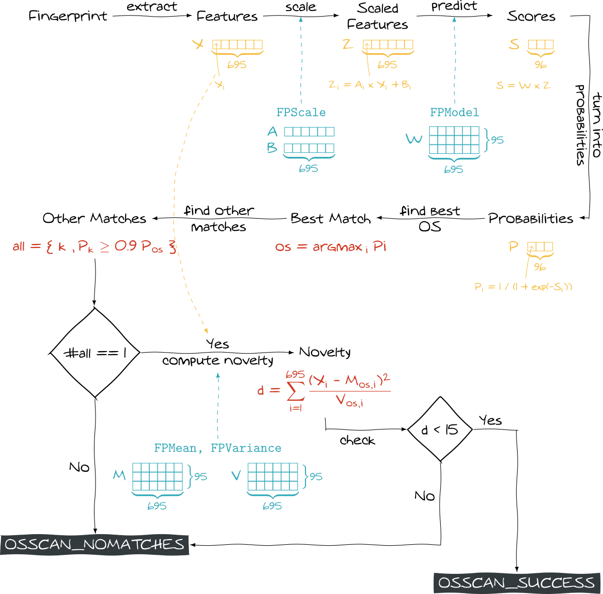
nmapDespite its practical efficiency, we can do a couple of remarks:
- The model (all the blue elements) is totally static, a bit crude (raw values) and hard to enrich by ourself.
- Some aspects are more about hacking: uncommon pipeline, use of hardcoded constants and strange choices (about the number of matches especially).
I personnally think that we could improve the whole detection engine (using also an ML approach for IPv4). The key elements would be to use a more flexible design and to set up a more “modern” detection workflow (to try it at least). I develop some of these ideas in the last paragraph.
Ideas to improve NMAP
The built-in nmap model is very powerful as it takes into account almost hundred OS. However it is static and possibly updated only when a new version is available.
Imagine you have fingerprints of very uncommon systems like SCADA or seldom firmwares. You have to submit this fingerprint to update the whole model (updating the model locally is rather hard). You possibly don’t want to share your fingerprints or even you are very motivated, it will take time as we can see in that post of Daniel Miller:
[…] integrating user-submitted fingerprints is a manual process that takes several weeks of dedicated time to accomplish each year. We (the Nmap developers) are always looking for ways to improve this process and make more frequent updates, but generally there are only 2 releases per year.
So the idea would be to have a more dynamic model that every nmap user can enrich (interactively for instance) and possibly share. A solution would be to have a fingerprint database. Yes, it already exists: /usr/share/nmap/nmap-os-db, but this is for IPv4 fingerprints. Moreover fingerprints should be stored directly as a feature vector. Thus, the model could be easily rebuilt by the user.
Furthermore, the current process computes the novelty of a new fingerprint but this piece of information is not exploited either while it could improve our detection engine.
Can we use a even more powerful workflow? It is hard to talk about the choice of the algorithms. The number of features is quite high (695), but even if liblinear is made for large scale datasets, I would rather have a look to other classifiers like Random Forest which does not need scaled data, may select the most relevant features and fits all the classes at the same time (no one-versus-all approach). About novelty detection, the computed distance is a bit uncommon. From the random forest classifier, it is possible to set a kind of “certainty threshold” below which the fingerprint is not classified. Another way would be to compute the Local Outlier Factor (LOF) to check if the fingerprint looks like its neighbours (but it requires several labeled samples).