13 minutes
Desktop Elements Detection Using Deep Learning
Notes
The original post (written with Joseph Paillard) has been published on the Amossys blog. Here, some elements related to the Amossys company (and not paramount on this blog) have been removed.

Context
This project has been carried out as part of the AI & Cyber challenge that took place during the European Cyber Week (ECW) 2020. This year, the challenge was to emulate human behavior on a computer. For that purpose, each team had to develop an agent that interacts with a machine via the VNC protocol (no running agent allowed on the target). Programs were then judged on the visual performance they provided and whether they tricked the jury or not.
This specific project was initially aiming at developing an autonomous agent capable of browsing a file explorer. Yet, we rapidly decided to consider the more general task of desktop component detection, which also embraces the detection of close buttons, mail icons etc. The main constraint was that the solution had to be generic, i.e. able to handle changes of Linux distribution and theme.
Strategy
Among the 5 human senses, sight is the most used during computer activity. Therefore, in order to emulate human behavior, it is relevant to try to replicate the human visual perception of the computer. Computer vision, a sub-field of artificial intelligence, was born in the 1960s to tackle this issue.
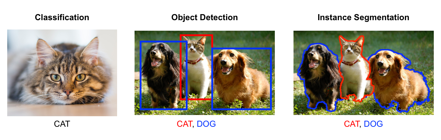
The goal is to identify desktop objects on screenshots along with their position (in order to generate a browsing activity). Among computer vision sub-fields, object detection is the most relevant since boxes are sufficient to segment the desktop components (geometrical shaped).
Methods for object detection generally fall into deep-learning-based approaches and are typically based on Convolutional Neural Networks (CNN). The following section describes what makes CNN different from other neural networks and why they are so efficient for computer vision tasks.
Convolutional Neural Networks (CNN)
A CNN is a deep neural network highly effective for computer vision tasks. The architecture of CNNs is bio-inspired and emulates the organization of the visual cortex. It is made of an assembly of convolution layers, pooling layers and fully connected ones.
A basic neural network is generally made up of a series of fully connected layers. In such layers each neuron is connected to all the neurons of the next layer and a weight is associated to each binding. These layers are used to learn features by changing the weights of the bindings between neurons during the training. But such networks turn out to be irrelevant for computer vision tasks for two main reasons :
- It requires a huge architecture to consider every pixel
- It removes spatial dependency between pixels
This is where convolution comes in, it aims at extracting dominant features that will help to characterize objects (e.g. edge detection, color detection… ). For that purpose, a filter is applied throughout the input image by applying matrix multiplications on small regions of the image and moving the next one with a certain stride.
The output of the convolution layer is called the feature map. Its size can be either smaller than the input or larger which is useful to decrease the computational power required. More complex transformations are also applied later on in the network (e.g. pooling, for more information refer to the sources section) but the key asset of CNNs is that hardly any pre-processing is required since it is handled by the convolution layers.
Model Selection
Even among CNN based algorithms, a wide range of architecture variations exists. They differ on accuracy, speed but also on computational power requirements which is crucial when working with resource constraints. All these aspects have to be taken into account so as to choose the most adapted algorithm.
Three models stand out in object detection regarding speed and precision:
- Region Proposals (Faster-R-CNN)
- You Only Look Once (YOLO)
- Single Shot MultiBox Detector (SSD)
Basically YOLO is the fastest while Faster-R-CNN is the most accurate (SSD lies in between). You can take a look at this post for a deeper analysis. In our approach, we have mainly worked with Faster-R-CNN since accuracy seemed to be the most relevant feature. Having a couple of predictions per second is enough to mimic human behaviour.
From the hardware point of view, a reasonable size GPU (GeForce GTX 1660 with 6 GB of RAM) allows us to load the model and to provide inferences at a speed of approximately 5fps.
Tailoring Faster-R-CNN to icon detection
Once a model has been selected it is not yet ready do be used. It still needs to be trained to the icon detection task as computer vision models are usually trained and evaluated on other kinds of objects (cats, dogs, pedestrians, cars…).
The problem is that training a computer vision model from scratch requires a huge dataset (millions of images) and a tremendous computational power, which is out of range for the vast majority of users. But all hope of success is not lost: transfer learning allows to train a model with the slightest effort by taking advantage of pre-trained models.
Fine-tuning
Fine-tuning is a quite efficient technique to tailor Faster R-CNN to our icon detection task. Instead of initializing the model randomly, we start from a model that has been pre-trained on a very large dataset (e.g. ImageNet, which contains 1.2 million images with 1000 categories). At this stage, the model is very efficient for common object detection. Training is then performed on the final layers while early ones are frozen. This is motivated by the observation that the early layers of a CNN contain more generic features (e.g. edge detectors or color detectors) that are useful to many tasks. Later layers of the CNN become progressively more specific to the details of the classes contained in the original dataset. For more details about Faster R-CNN architecture, refer to original paper. As a result, the number of parameters to optimize is widely reduced and frozen ones are already close to their optimal value.
In PyTorch, a pre-trained Faster R-CNN model (with a resnet50 backbone) can easily be loaded using the torchvision package:
import torchvision

model = torchvision.models.detection.fasterrcnn_resnet50_fpn(pretrained=True)
Obviously, this model is made for a given number of classes. When you want to adapt the algorithm to a different number of classes, you have to modify the last layer:
from torchvision.models.detection import fasterrcnn_resnet50_fpn
from torchvision.models.detection.faster_rcnn import FasterRCNN, FastRCNNPredictor

def get_model(num_classes: int) -> FasterRCNN:
    # load an instance segmentation model pre-trained on COCO
    model = fasterrcnn_resnet50_fpn(pretrained=True)

    # get the number of input features for the classifier
    in_features = model.roi_heads.box_predictor.cls_score.in_features

    # replace the pre-trained head with a new one
    model.roi_heads.box_predictor = FastRCNNPredictor(in_features, num_classes)

    return model
To check which parameters will be optimized, we can have a look
to their require_grad attribute.
Each parameter that has require_grad set to True will be updated whenever the optimizer function is called (i.e. a gradient descent step is performed). In our case it is easy to check which part of the model is frozen:
for name in model.named_parameters():
    if param.requires_grad:
        print("{0} requires grad".format(name))
    else:
        print("{0} doesn't requires grad".format(name))
backbone.body.layer1.X.convX.weight doesn't requires grad
backbone.body.layer2.X.convX.weight requires grad
...
rpn.head.conv.weight requires grad
roi_heads.box_head.XXX requires grad
roi_heads.box_predictor.bbox_pred.weight requires grad
Here we can see that the first convolution layer is frozen while next ones are modified during the fine-tuning step.
Dedicated dataset
A relevant dataset is often the keystone of success in machine learning. In particular, identifying every object on the screenshot is paramount. Even though fine-tuning requires a minimum amount of data, an effort is required to create the dataset for our purpose.
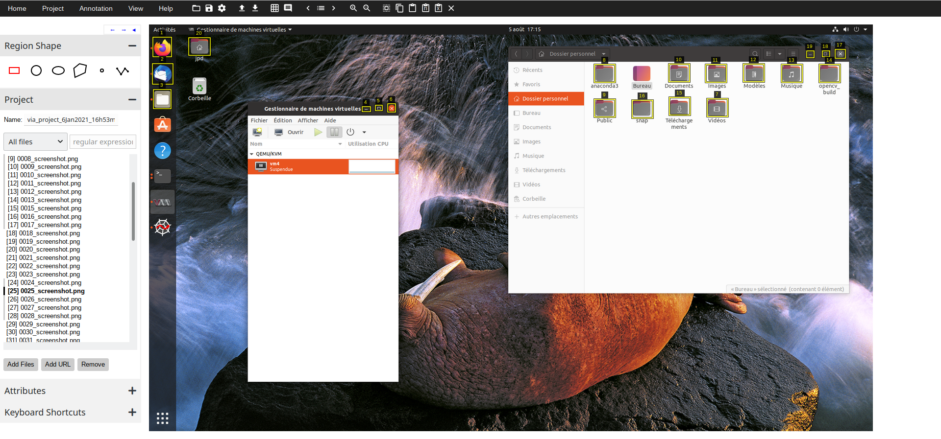
First, several screenshots (about 100) from various [Linux] environments have been taken. Then, each image has been annotated with bounding boxes related to the classes we want to detect (about 10 at the beginning). For image annotation, we use VGG annotator, which is a simple and easy-to-use HTML application (see below).
Once the images are treated, we can export the annotations to a json file which is structured as follows.
...
"0061_screenshot.png708446": {
    "file_attributes": {
        "distribution": "ubuntu"
    },
    "filename": "0061_screenshot.png",
    "regions": [
    {
        "shape_attributes": {
            "name": "rect",
            "x": 111,
            "y": 36,
            "width": 47,
            "height": 42
        },
        "region_attributes": {
            "Icon": "folder"
        }
    },
    {
        "shape_attributes": {
            "name": "rect",
            "x": 14,
            "y": 109,
            "width": 45,
            "height": 45
        },
        "region_attributes": {
            "Icon": "folder"
        }
    },
 ...
 ],
We can easily identify the bounding boxes (shape_attributes) and their label (region_attributes).
Training in practice
To train Faster-RCNN on our custom dataset we need two elements:
- a data-loader to feed data into the CNN
- an optimizer to modify the CNN parameters so as to perform the best detection
Data-loader
To feed some data to our Faster R-CNN, we mainly need a class respecting a basic interface.
It must bridge between the json given by VIA and the pytorch dataset interface.
In our case, its structure is given below.
class ScreenDataset:
    def __init__(self,
                 root: str,
                 transforms: Callable,
                 json_file: str):
        ...

    def __getitem__(self, idx : int):
        """
        Return the idx-th image (internally transformed) and its annotations (n boxes),
        following the following structure:

        target = {
            'boxes': [n x 4 tensor],
            'labels': [n x 1 tensor],
            'scores': [n x 1 tensor],
        }
        """
        ...
        return img, target

    def __len__(self):
        """
        Return the number of images in the
        root directory
        """
        ...
The initialization function checks the images located in the given root directory.
The provided transforms function is a common tool to correctly shape the input image to the CNN.
Finally, the json_file is the annotation file.
This object needs two additional methods to be wrapped in a more generic PyTorch DataLoader (allowing batch selection, shuffling etc.).
In details, the function __getitem__ selects an image, transforms it and parses the json file to output the
annotated boxes (target).
dataset = ScreenDataset(
    root="/path/to/images",
    transforms=fun,
    json_file="/path/to/file.json")

data_loader = torch.utils.data.DataLoader(
    dataset=dataset,
    batch_size=5,
    shuffle=True)
Optimizer and hyper-parameters
PyTorch proposes several optimizers. In our case, we use the classical stochastic gradient descent (SGD) which gives rather good results.
# get the parameters to optimize
params = [p for p in model.parameters() if p.requires_grad]
# init the oprimizer
optimizer = torch.optim.SGD(params, lr=0.005, momentum=0.9)
In Machine learning, the training phase aims at optimizing the parameters of a model. Taking a step back, the training process also has parameters that can be optimized in order to improve the efficiency of the training. These are called hyper-parameters and are usually defined by the user.
First of all, it should be understood that this choice is likely to be constrained by computational power, data and time limitation. The three main hyper-parameters that can be adapted are the following:
- number of epochs: The number of forward passes for each image of the dataset
- batch size: the number of training samples (here images) to work through before performing a backward pass.
- learning rate: the size of the step taken at each gradient descent.
The number of epochs depends on the dataset and the time you have to train the model. If you have a very rich dataset, a small number of epochs can be enough to train a good model. However, the model will overfit at a moment if it learns too much from the training set (the model cannot generalize).
In order to obtain a consistent approximation of the gradient of the loss function, it must be calculated over a large enough batch. If the batch size is too small, gradient descent steps are more exposed to randomness and training may thus be longer. Nevertheless, with a smaller batch size, the memory of the GPU is less monopolized and the parameters of the model are updated more frequently (which may therefore reduce the training duration). Hence, a trade-off has to be found between precision (higher with larger batch size) and speed (shorter with frequent parameters updates and thus smaller batch size).
Finally, the learning rate is a pure optimization parameter as it corresponds to the step length taken after every batch. A small value means that the optimization is cautious (slow but sure) although a high value tends to accelerate the convergence with a risk to move away from optimum regions.
Other parameters also exist and should be carefully chosen.
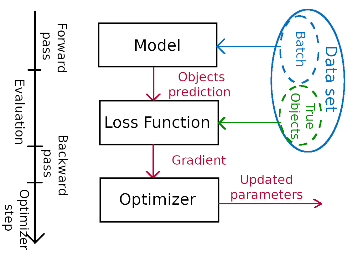
Training pattern
Now we have all the material to train our CNN. This stage includes 4 stages:
- forward pass (prediction)
- evaluation (loss calculation)
- backward pass (gradients calculation)
- optimizer step (gradient descent)
In practice, we merely need to loop over the data. A single epoch may look like this:
for images, targets in data_loader:
    # here we have a batch of images
    # and the bounding boxes (targets)

    # zero the parameter gradients
    optimizer.zero_grad()

    # compute the loss (forward pass)
    loss = model(images, targets)
    # gradient backpropagation
    loss.backward()
    # weights update
    optimizer.step()
Now, lets zoom in on Faster R-CNN:
- During the forward pass, the model is fed with a batch of images and returns the objects detected in those images along with their bounding boxes and a confidence score for each prediction. The output looks like this:
model.eval()
print(model(img))

{'boxes': tensor([[1668.7316, 271.4885, 1753.3470, 359.6610],
[ 973.9626, 402.9771, 1059.8567, 490.3125],
[1669.7742, 403.1881, 1754.4435, 490.4958],
[ 973.8992, 271.6441, 1059.7217, 359.6740]], device='cuda:0'),
'labels': tensor([7, 7, 7, 4], device='cuda:0'),
'scores': tensor([0.9905, 0.6706, 0.4652, 0.3768], device='cuda:0')}
- Afterwards the loss is calculated. A loss function takes the (output, target) pair of inputs, and computes a value that estimates how far away the output is from the target. The relevant loss function for object detection is intersection over union (IoU): it compares the ground truth object position with the predicted bounding box.
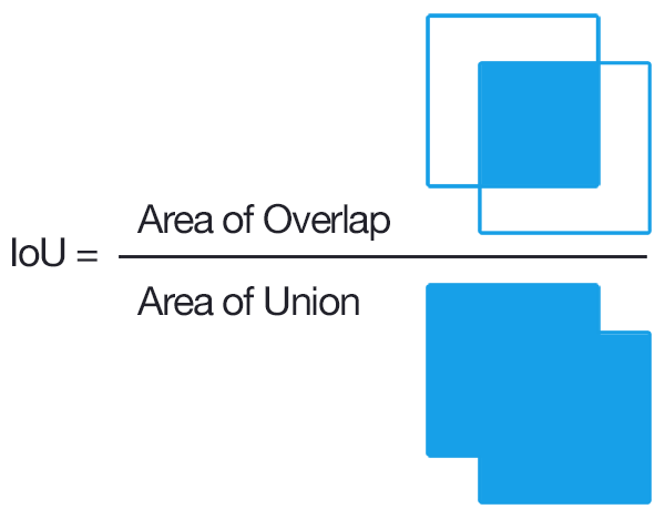 Intersection over Union
 - During the backward pass, the gradient of the loss function is computed with back propagation.
- Finally the optimizer performs a gradient descent in order to optimize the parameters of the model (SGD).
Our model needs about 10-15 minutes to train (100 images, 15 epochs, 2 images batch) with a GTX 1060 6GB.
Results
Since the ECW challenge, we have been developing the desker library that aims at implementing several desktop elements detection routines. Our Faster R-CNN model is available through this library, so you can test it!
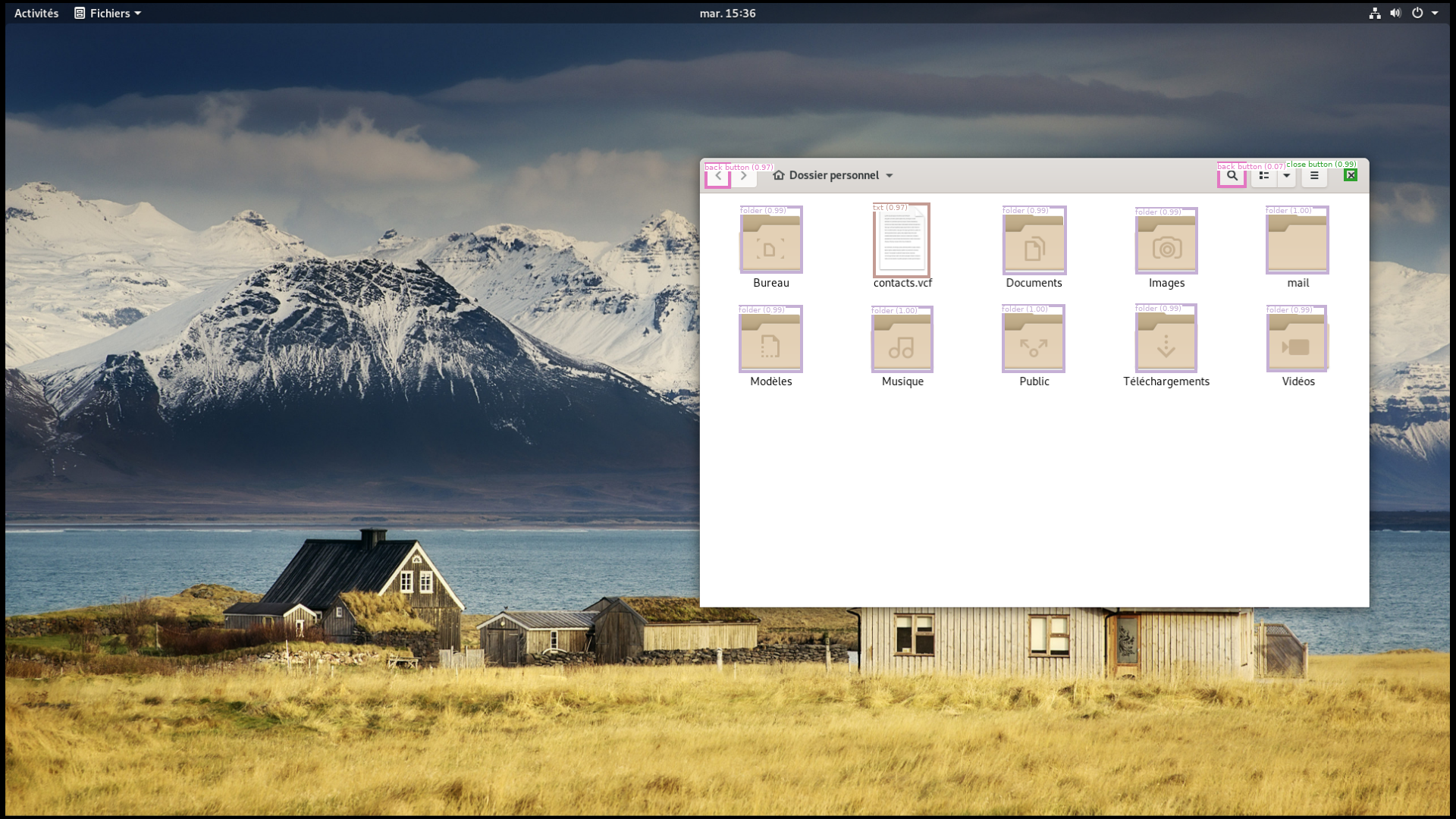
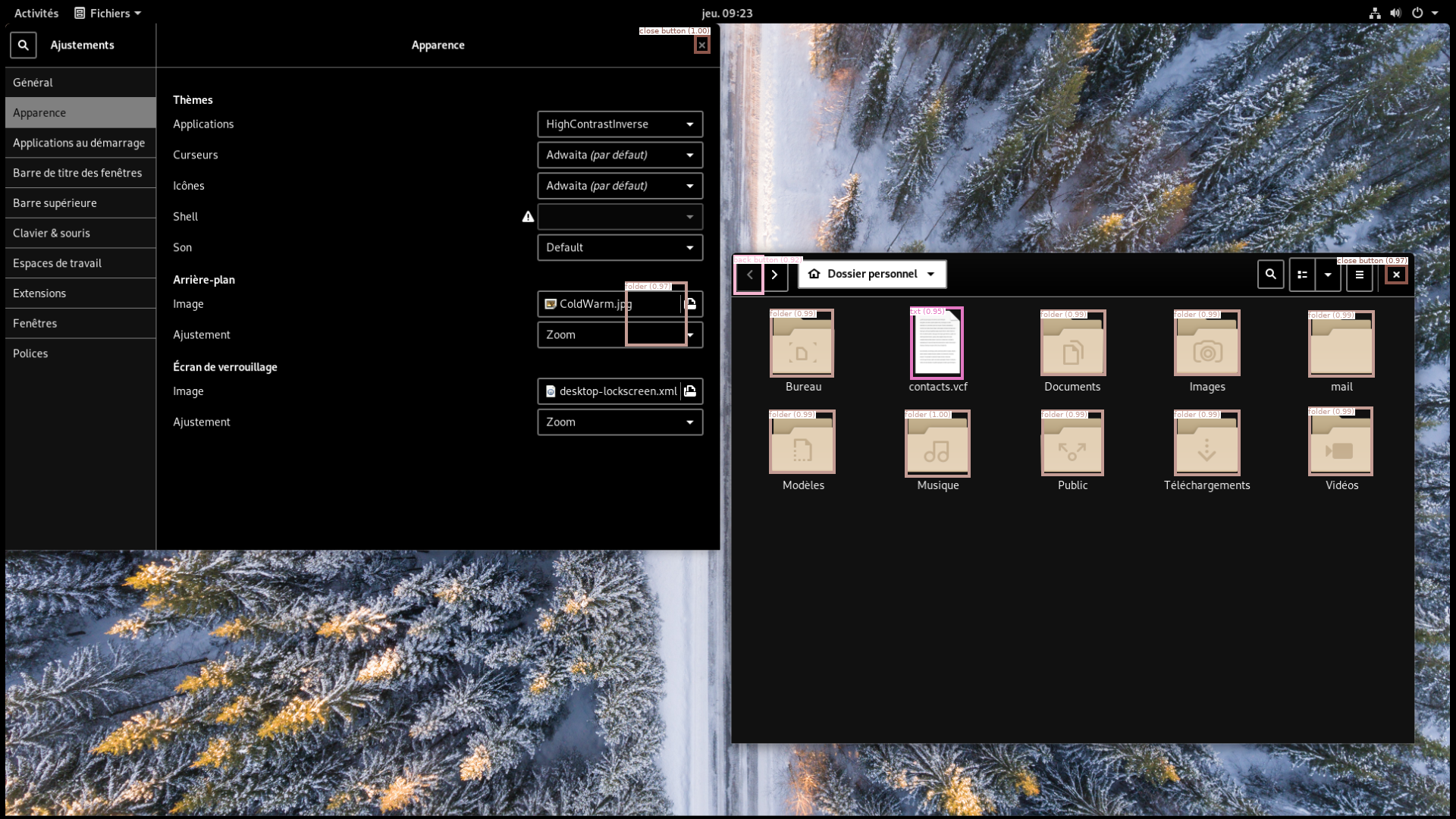
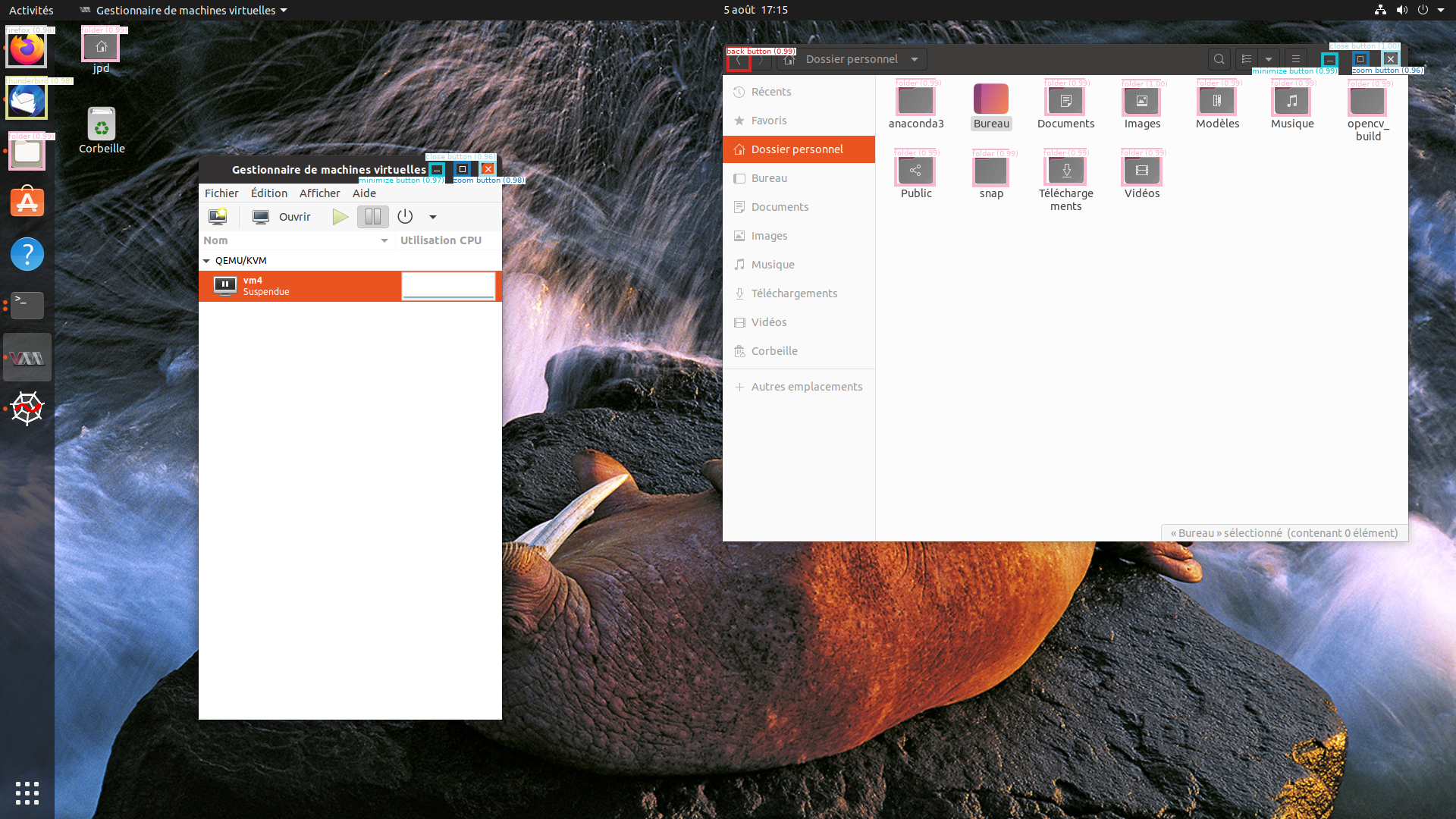
Here you can look at the results given by our trained model on various test images.
 |  |
 |  |
 |  |
Conclusion
Computer vision is certainly a useful tool to identify relevant objects on a screen. This step is fundamental to generate human-like computer activity.
Moreover, object detection can be associated with optical character recognition (OCR) and other image processing techniques to analyze the text on the same screenshots. Such information could produce even more realistic actions (browsing specific folders, clicking on links…). Some of these methods can notably be found in desker.
Extra: exploring gradient accumulation
Even with the slightest training phase, several memory issues may arise and hamper the training process. This section introduces a solution to overcome the famous “out of memory” issue that occurs when the GPU lacks RAM.
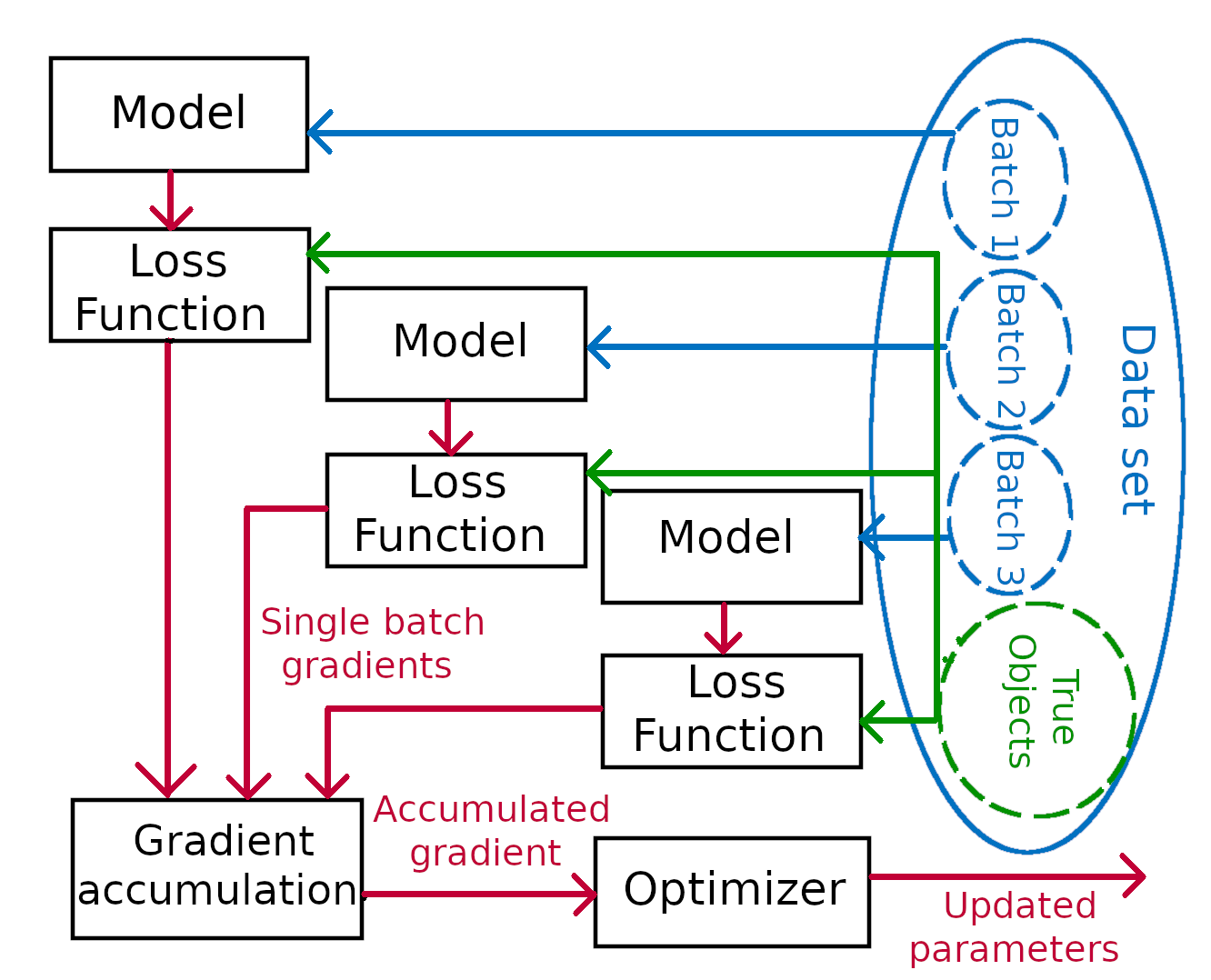
It is worth noticing that the batch size corresponds to the number of images that will be loaded simultaneously on the GPU. Therefore besides slowing down the training process, a limited computational power also prevents from reaching a good approximation of the gradient and thus hampers the quality of the training. However the gradient accumulation method allows to make up for the lack of RAM. To cope with the constrained memory, a given batch is divided in mini-batches which are loaded sequentially on the GPU and forward passed in the model. Then, after each step, the gradient is calculated with back propagation but the parameters of the model are only updated after a given number of steps (equal to the number of mini-batches in a batch). Even if the sum of the gradients is clearly not equal to the gradient of the larger batch, it offers a better approximation while avoiding out of memory errors.
To experiment it we used the following hyper-parameters.
| Hyper-parameter | Value |
|---|---|
| batch size | 3 |
| number of epochs | 10 |
| learning rate | 0.005 |
| learning decay | 0.0005 |
The learning decay is a hyper-parameter that reduces the size of the gradient descent step after each epoch adjust the learning speed (at the end of the learning, only tiny modifications are required). Results are presented below.
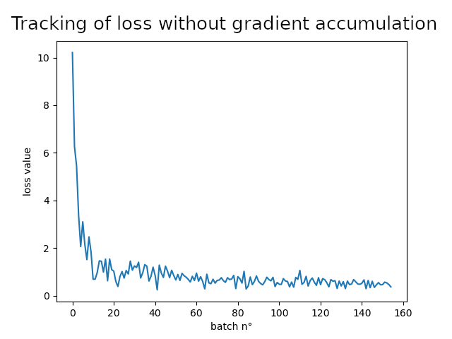
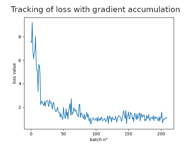
With such hyper-parameters gradient accumulation doesn’t seem to make any difference, chances are that it is due to the small size of the dataset. Nevertheless, the model converges and makes satisfying predictions.
Sources
- https://en.wikipedia.org/wiki/Convolutional_neural_network
- https://towardsdatascience.com/a-comprehensive-guide-to-convolutional-neural-networks-the-eli5-way-3bd2b1164a53
- https://medium.com/@jonathan_hui/object-detection-speed-and-accuracy-comparison-faster-r-cnn-r-fcn-ssd-and-yolo-5425656ae359
- https://gitlab.com/d3sker/desker